
Machine learning (ML) in Mechanics is a fascinating and timely topic. This article follows from a kind invitation to provide some thoughts about the use of ML algorithms to solve mechanics problems by overviewing my past and current research efforts along with students and collaborators in this field. A brief introduction on ML is initially provided for the colleagues not familiar with the topic, followed by a section about the usefulness of ML in Mechanics, and finally I will reflect on the challenges and opportunities in this field. You are welcome to comment and provide suggestions for improvement.
1. INTRODUCTION (for people not familiar with ML)
ML has been around for more than 60 years, alternating through periods of euphoria and skepticism – see timeline in https://www.import.io/post/history-of-deep-learning/. In the last decade(s), however, the field has become much more accessible to non-specialists due to open source software written in general-purpose programming languages (e.g. Python). Unsurprisingly, early adopters of ML are found in fields with open databases gathering vast amounts of data from simulations or experiments, such as bioinformatics (e.g. https://www.ncbi.nlm.nih.gov/), chemistry (e.g. https://pubchem.ncbi.nlm.nih.gov/) and materials science (e.g. http://oqmd.org/ and http://aflowlib.org/). Yet, ML can impact any scientific discipline where enough data about a problem is available. Mechanics is no exception, despite its specific challenges (see section 3).
For the purposes of this discussion, I will focus on two branches of ML: supervised learning (regression and classification), and unsupervised learning (clustering). The third main branch, reinforcement learning, is not discussed here.
If you are new to ML, and you want to get some hands-on experience, I recommend to start with Scikit-Learn (https://scikit-learn.org/) – no conflict of interests in this recommendation. Its user interface is simple, as it is written in Python, and the documentation is very useful as it starts with the most restrictive algorithms (e.g. linear models such as ordinary least squares) and ends with the least restrictive ones (e.g. neural networks). This is important because it provides the correct mindset when applying ML algorithms to solve a problem: in the same way that you don’t use an airplane to go from the living room to the kitchen; you probably don’t want to use a neural network to discover that your data is described by a second order polynomial. In addition, Scikit-learn’s documentation also has a simple introduction for each algorithm and multiple examples (including source code). This allows you to try different algorithms even before you understand their inner workings and why some algorithms are better choices than others for a given problem.
I created a script with simple examples that requires Scikit-learn and Keras (https://keras.io/) and that can be used to replicate the figures of this section and get more information about error metrics. The script is callend "Intro2ML_regression.txt" and it requires that you have Scikit-learn and Keras installed in your system. Please chance the extension from .txt to .py to run it. Keras is a high-level Application Program Interface (API) to create neural network models. It interfaces with powerful ML platforms with optimized performance, TensorFlow or Theano, while keeping them user friendly.
1.1. Supervised learning: regression
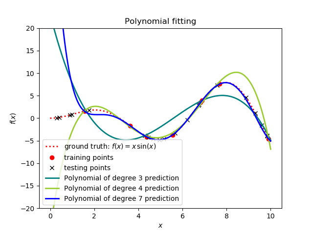
Even if you are not familiar with ML, as a researcher/practitioner in engineering you probably faced simple regression tasks (curve fitting) in which you were given a set of discrete points (training data) for which you want to find a continuous function (model) that interpolates all the points or that describes the general behavior of the data by smoothing it (e.g. least squares regression). The outcome of this task is a parametric function that describes your data, e.g. y=ax3+bx+c, and that should predict the data points that were not included in the fitting process (testing data). Let’s consider an example: the figure below shows the best fit of three different polynomials using 8 training points (red dots). The red dashed line represents the true function (to be discovered) and the black crosses represent testing points within that function that were not used for fitting the polynomials. Note that the polynomial of degree 7 is interpolatory, while the other two polynomials are not (smoothing the data). The quality of the prediction is then assessed by simple error metrics, e.g. mean least squares, calculated between the prediction of the model at the test points. For example, the test points close to x=0 in the figure below are very far from the predictions provided by the three polynomial models, leading to a large mean squared error.
Similarly to polynomial fitting, ML algorithms are also capable of regression via supervised learning. However, ML algorithms create models that are not parametric. In other words, these algorithms have so many parameters that it does not make sense to try to obtain the underlying analytical expression. Therefore, people colloquially refer to ML models as black boxes: they are predictive, but we don’t know the analytical form of the model. We lose insight, but we gain very powerful regression tools.
1.1.1. Choosing an ML algorithm
To illustrate the argument of not using an airplane to go from the living room to the kitchen, consider two classic ML algorithms:
Neural Networks (NNs) in their non-Bayesian formulation: the quintessential ML algorithm, based on millions of combinations of simple transfer functions connecting neurons (nodes) that depend on weights. Training involves finding this vast amount of weights such that they fit the data accordingly. Neural networks are very simple algorithms, so they are extremely scalable (they can easily deal with millions of data points). However, as you can imagine, training is not a trivial process because of the overwhelming possibilities for finding the weights of every connection.
Gaussian Processes (GPs): a Bayesian or probabilistic ML algorithm, meaning that it predicts the response as well as the uncertainty. This algorithm has outstanding regression capabilities and, in general, is easy to train. Unfortunately, this algorithm is poorly scalable, so it is limited to small datasets (approximately 10,000 points).
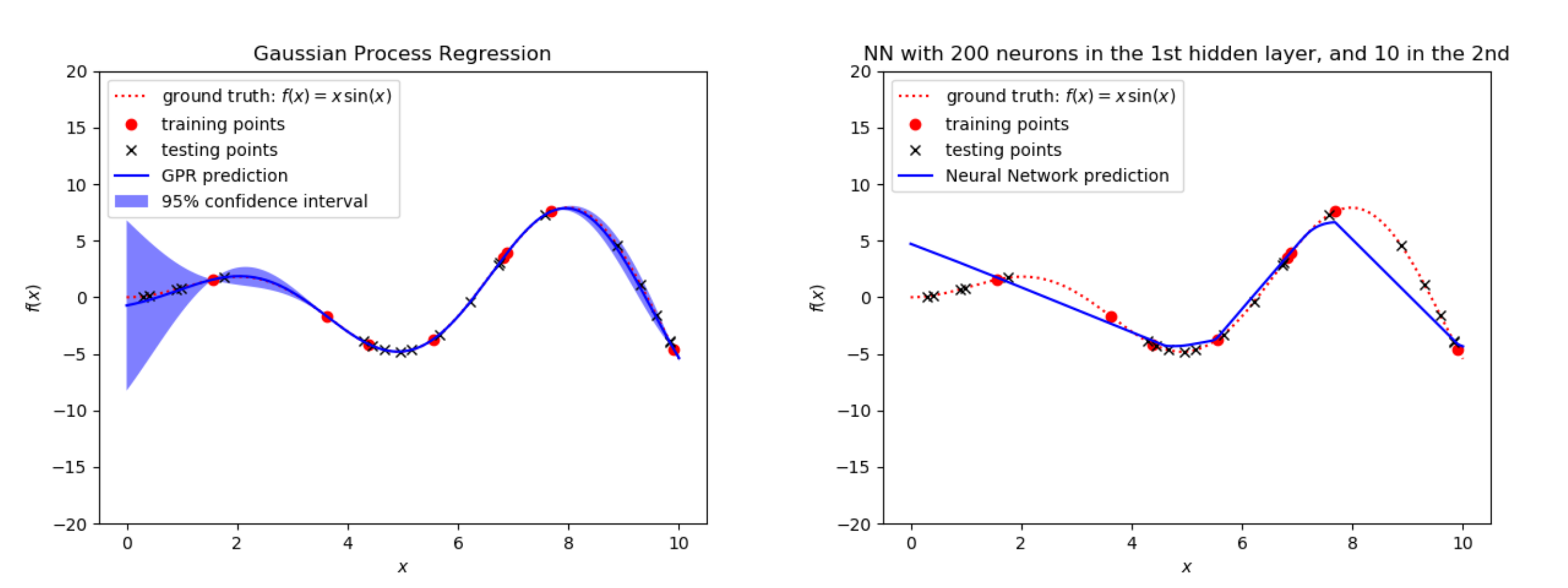
The figure below shows the result of training GPs and NNs for the same training data used above for polynomial fitting. As can be observed, GPs provide an excellent approximation of the function x*sin(x) even when using only 8 points, and they also quantify the uncertainty away from the training data. Yet, NNs are much harder to train on such a scarce dataset. In the script made available here, there is a grid search that helps finding reasonable parameters (neurons, epochs, etc.) for the neural network via cross validation, but as you can try by yourself, finding an appropriate model is not trivial. The script also includes much more information than what I am covering here, such as the loss obtained on the training and test data with the number of epochs, and the mean squared errors for the three approximation algorithms. The main point here is to illustrate my airplane analogy: NNs are in general not the best choice to approximate low dimensional and scarce data. Note, however, that both GPs and NNs approximate the function clearly better than polynomial regression.
1.1.2. Do we know a priori if there are “enough” training points?
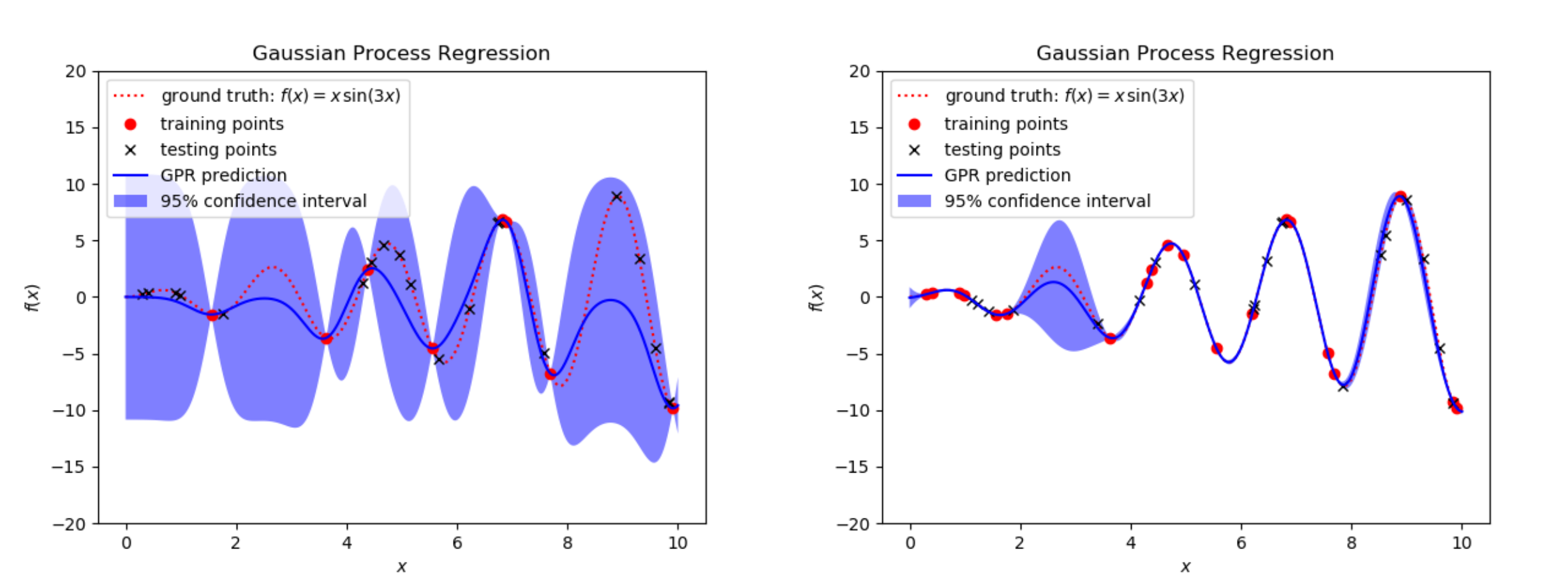
No. Consider a second example where the function to discover is now x*sin(3x) within the same domain. If we use 8 training points, as we did for finding x*sin(x), our approximation is obviously worst, as seen in the figure below. So, we need more training data to approximate this new function with similar quality. Hence, we only know that we have enough training data by iteratively assessing the error of our approximation against the test data. We stop increasing the training data size when the error converges to a reasonable value (or when you don’t have any more data!). In practice, the training data size may need to be very large when our problem has many input variables due to the curse of dimensionality: every additional input variable causes an exponential growth of the volume that needs to be sampled. This can be a strong limitation because we may not have thousands or millions of training datapoints required for appropriate learning.
1.1.3. What happens if my data is noisy or uncertain?
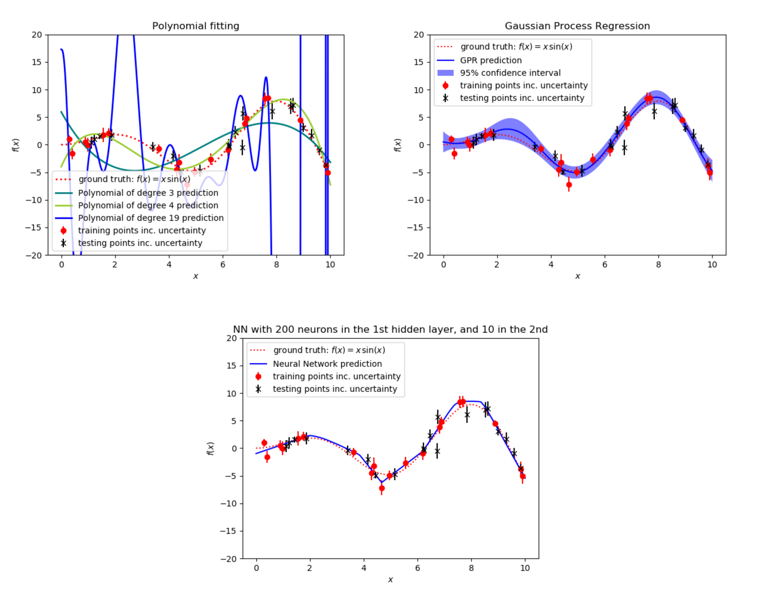
Noisy datasets are very common in Engineering. Data coming from experiments is often dependent on environmental fluctuations, material defects, etc. Note that even when the data comes from simulations, datasets can still be noisy (stochastic). For example, simulations of structures undergoing buckling depend on the geometric imperfections considered in the model. If these imperfections are sampled from a statistical distribution, then the properties will not be deterministic. The figure below illustrates the nefarious effects of stochasticity. The data is generated by perturbing the same x*sin(x) function but now we perturb it with Gaussian noise where (twice) the standard deviation is represented by the vertical bars in the data. As seen in the figure, the polynomial of degree 19 (interpolatory) suffers from severe overfitting, while GPs and NNs can be trained to predict the response appropriately. However, NNs need to be trained ensuring that overfitting does not happen, which in practice occurs by training via cross validation and observing the evolution of the loss data in both the training as well as the testing data.
1.1.4. What is the difference between ML and Optimization?
ML aims at learning a model that describes your entire dataset and predicts the response everywhere, whereas optimization aims at finding the optimum point, i.e. it does not care about regions that are far from the optimum. In principle, if you just want to find the optimum once, you should not need to use traditional ML algorithms, as direct optimization is likely to be faster. However, sometimes ML can help the optimization process because it can provide a surrogate model, i.e. a model that describes the data reasonably well and that is differentiable. An easy example to visualize the benefits of having a surrogate model from ML is to consider the above noisy dataset. ML algorithms can learn the underlying function and disregard the noise (smoothen the response surface) by treating it as uncertainty, which significantly facilitates the task of finding an optimum. This has the added benefit of enabling the use of gradient based optimization methods! However, there is a trade-off. If you spend a lot of computational effort in learning regions of the surrogate model that are far from the optimum, you are wasting resources that could be better exploited by the optimization algorithm alone. Hence, the trade-off is between exploration of new regions and exploitation of regions where the likelihood of finding the optimum value is high.
1.2. Supervised learning: classification
Classification is probably the most widely known task in ML. Instead of learning a continuous model, the ML algorithm learns discrete classes. Having understood how to train for regression tasks, classification is not significantly different. The typical example is learning from (many) images of cats and dogs how to classify an unseen image as a cat or as a dog. Training occurs in a very similar way as what was described in 1.1. As referred in section 2, classification can be useful to determine the bounds of the design space that contain interesting information (where you can perform optimization or regression).
1.3. Unsupervised learning
These ML algorithms attempt to find patterns in data without pre-existing labels. Clustering is a typical task of unsupervised learning, where the algorithm finds groups of points that have similar characteristics according to a chosen metric. In mechanics, people familiar with Voronoi diagrams should have a good idea about how clustering works, as this algorithm for the basis for an important unsupervised learning method called k-means clustering. The next section also provides an example from our work that illustrates the usefulness of unsupervised learning in mechanics.
2. IS ML USEFUL IN MECHANICS?
ML is especially useful when we have access to large databases for the problems of interest and when the analytical solution is not known. In mechanics, these can be difficult conditions to meet, as it will be discussed in Section 3. Yet, there are multiple situations where ML algorithms can be very useful in solving Mechanics problems. I will highlight a few of our examples and provide links to the codes that can be used for different problems. Our group is working towards making these codes more transferrable and more user-friendly. I also invite you to share your own examples in the comments below.
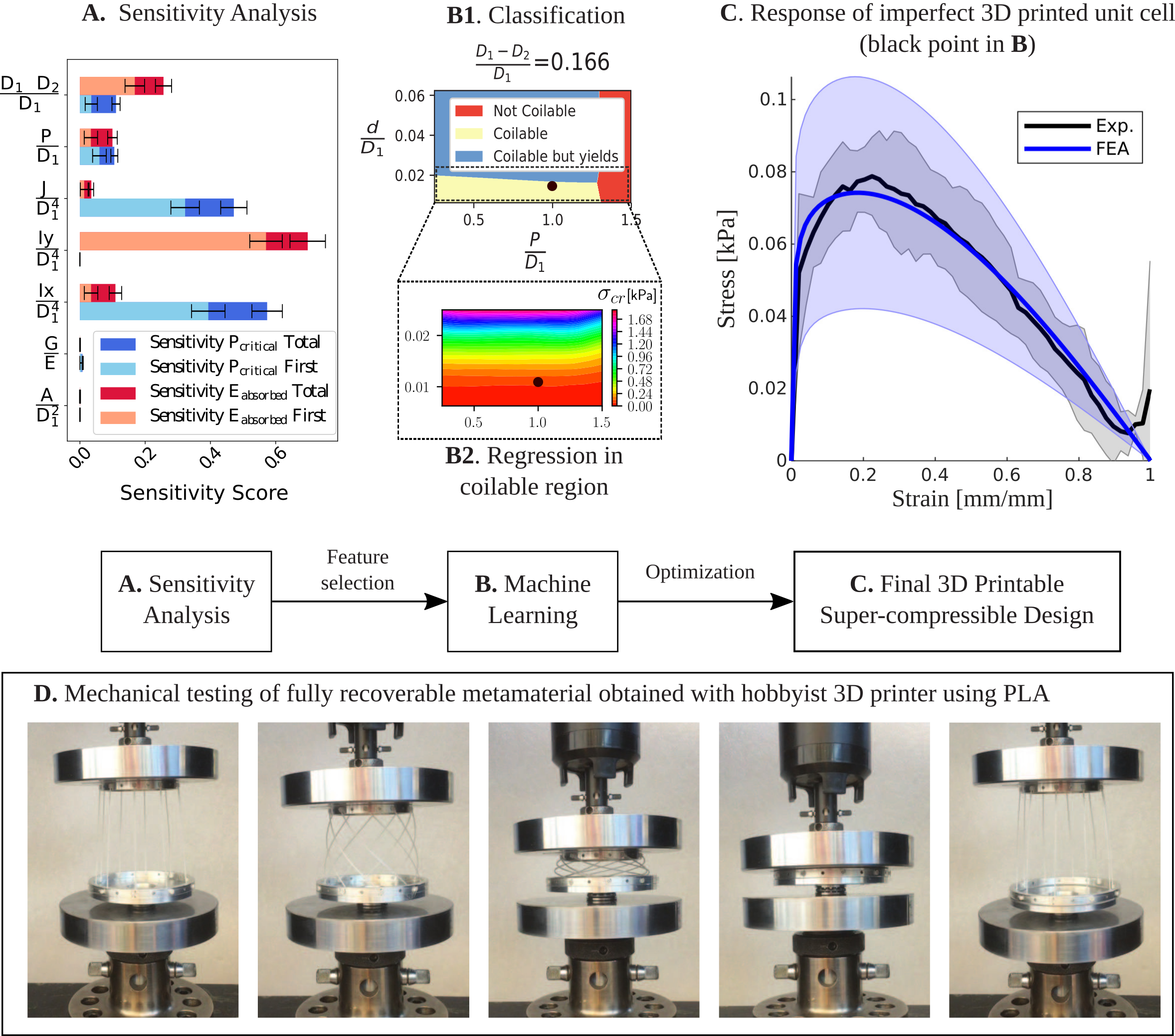
2.1. Classification and regression: Metamaterial design assisted by Bayesian machine learning [1]
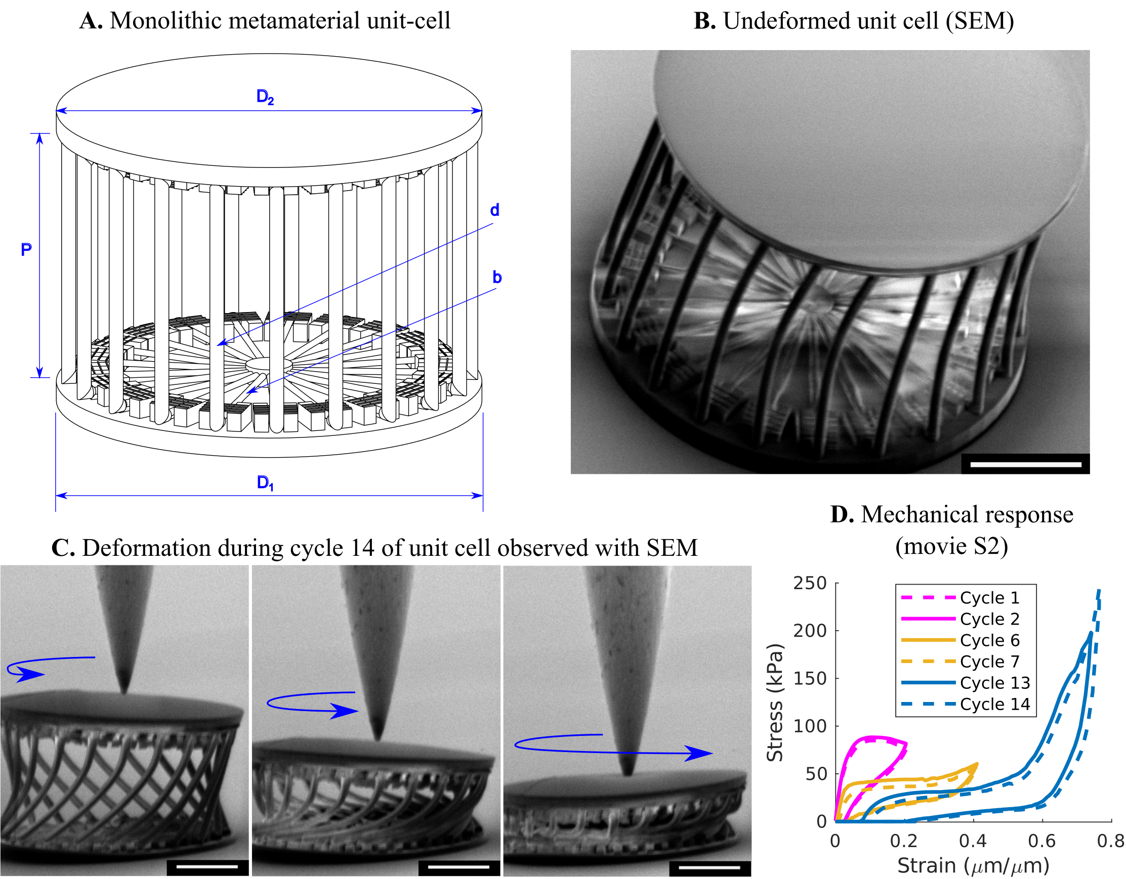
Metamaterial design is primarily a geometric exploration aiming at obtaining new material properties. Mechanical metamaterials tend to explore extreme buckling and postbuckling behavior, which means that the properties of interest are sensitive to geometric imperfections. Designing under these circumstances is challenging because the database includes uncertain properties (noise), and the regions of interest can be narrow (in the figure above, the yellow region corresponds to the only region where the metamaterial topology is classified as reversibly supercompressible). As illustrated at the end of section 1, ML is particularly suitable for learning under uncertainty, and in the case of Bayesian ML it can even predict the uncertainty of the model predictions. This facilitates the navigation of the design space, and the subsequent robust optimization. Using a new Bayesian ML method [2] that extends the traditional Gaussian Processes to larger database sizes (>100,000 training points), we showed that a metamaterial could become supercompressible [1] by learning directly from finite element simulations and without conducting experiments at the metamaterial level (only characterizing the base material). The supercompressible metamaterial was then validated experimentally a posteriori by mechanically testing 3D printed specimens created with brittle base materials at the macroscale (figure above) and micro-scale (figure below).
The code used in this work is available: https://github.com/mabessa/F3DAS
General purpose video about this work: https://www.youtube.com/watch?v=cWTWHhMAu7I
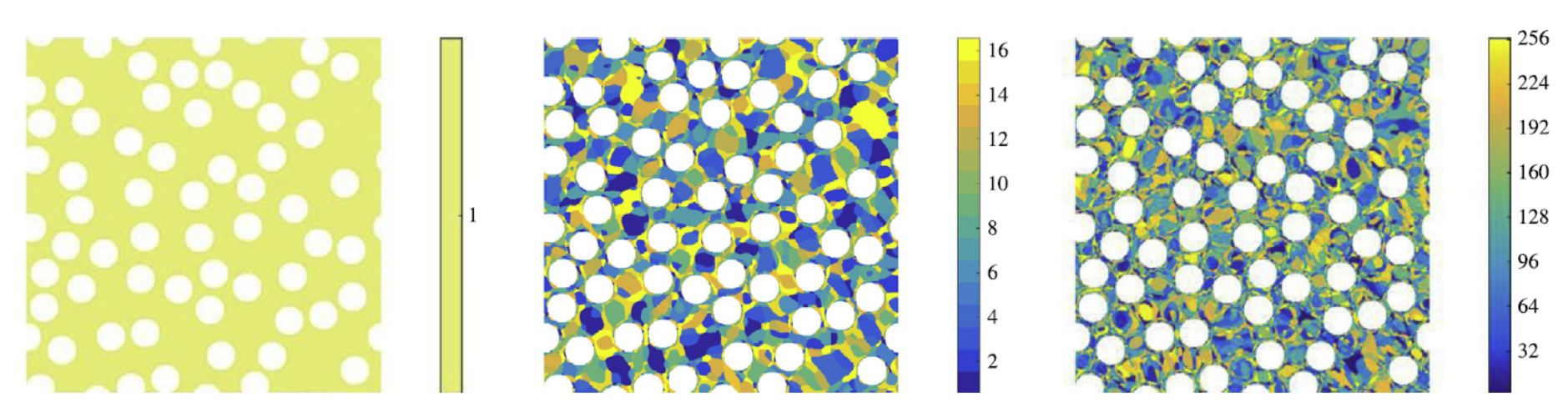
2.2. Clustering: Data-driven modeling of plastic properties of heterogeneous materials [3,4]
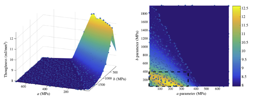
In work developed in collaboration with Zeliang Liu and Wing Kam Liu [3], we created a new numerical method called Self-consistent Clustering Analysis (SCA) where the computational time of simulations of plastic heterogeneous materials with damage is reduced from 1 day in a super-computer to a few seconds/minutes. One of the key ideas of this method was to use clustering ML algorithms to compress the information of heterogeneous materials by grouping points that have similar mechanical behavior. This enabled the creation of databases of adequate size to model the variation of toughness of these composites via a data-driven framework we created in [4]. The code for the data driven framework is similar to the previous one (F3DAS), but it is tailored to creating representative volume elements of materials: https://github.com/mabessa/F3DAM
The figure below shows the variation of composite toughness for different ductile matrix materials that was learned with the data-driven framework. In the figure each blue dot represents a simulation obtained by SCA.
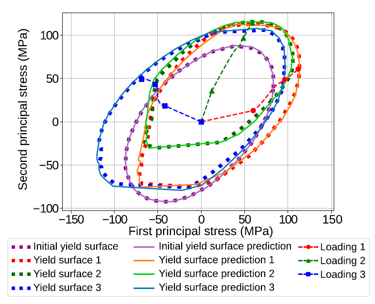
2.3. Deep learning: Predicting history- or path-dependent phenomena with Recurrent Neural Networks [5]
One difficulty we faced in [4] was the inability to learn history-dependent or path-dependent phenomena using ML algorithms. This is non-trivial because the ML map that needs to be built between inputs and outputs is no longer unique, i.e. there are different paths to reach the same state and the state depends on the history of states that occurred previously. However, in the work developed in collaboration with Mojtaba Mozaffar and others [4], we showed that recurrent neural networks (RNNs) had the ability to learn path-dependent plasticity. In principle, any irreversible time- or path-dependent process can be learned by RNNs or an equivalent algorithm, although the training process can be difficult. The same base code as in [4] was used here, , this time using RNNs as the ML algorithm: https://github.com/mabessa/F3DAM
The figure below shows the yield-surface evolution under different deformation conditions and paths. Finite element predictions are shown in dotted lines, while the deep learning predictions are shown in solid lines. Note the distortion of the yield surfaces with different loading paths, which is predicted by the RNNs.
3. CHALLENGES AND OPPORTUNITITES
There are significant challenges and opportunities within the field of ML and Mechanics. Coincidentally, last week there was a CECAM-Lorentz workshop co-organized by Pedro Reis (EPFL), Martin van Hecke (Leiden/AMOLF), Mark Pauly (EPFL) and me (TU Delft) where there was an open discussion about this topic. The following points reflect part of the discussions, but they result from my own views and personal perspective on the topic. I am happy to expand this list based on feedback:
1. High-throughput experiments: data hungry ML algorithms create challenges to experimentalists because they promote the creation of high-throughput experiments. Furthermore, open sharing of data via centralized repositories may become a necessity.
2. Improved efficiency of complex simulations: there are many simulations whose high computational expense still impairs the use of machine learning and data-driven methods. In solids, fracture and fatigue remain a challenge, while in fluids one of the concerns is turbulence. Development of new reduced order models [3,6,7] is fundamental for advancements in the field.
3. Physics-informed ML: an alternative to creating more data is to encode prior information in ML algorithms based on known physics, such that they require less data to learn [8,9]. For example, Thomas et al. [8] encoded rotation- and translation-invariance into neural networks, which facilitates learning in different settings (think about molecules rotating in an atomistic simulation).
4. Uncertainty quantification for very large dimensional problems: Zhu and Zabaras [9] have shown how Bayesian deep convolutional encoder-decoder networks are powerful methods for uncertainty quantification in very large dimensional data. This can open new ways of dealing with large data while still quantifying uncertainty.
5. ML to discover new laws of physics: Smidt and Lipson [10] have shown that genetic programming symbolic regression can learn Hamiltonians and Lagrangians by observing different systems, such as a swinging double pendulum. This is a different approach to artificial intelligence, where evolutionary algorithms are used to create equations (eliminating the “black box”). Brunton et al. [11] developed a fast alternative by limiting the form of the governing equations and leveraging sparsity techniques. These and other efforts towards learning the underlying equations that describe a physical process are important because such laws are extrapolatory, which is not quite the case for the other ML techniques.
6. Reinforcement learning and Bayesian optimization: there are techniques where ML algorithms are used to perform optimization by avoiding pre-sampling of the design space. Online Gaussian Processes [12], for example, are a type of Bayesian optimization algorithm that sits in between ML and Optimization. They are capable of finding a balance between exploration and exploitation in an attempt to quickly reach a global optimum.
7. Mechanics to improve the understanding of ML: a puzzling article by Geiger et al. [13] highlights that it is not just ML that can help Mechanics, but in fact Mechanics can help ML. Granular media may help uncover properties of deep neural networks! Certainly, there are many more interesting directions to pursue following other recent works [14-17], among many others. I apologize in advance for not including more articles from other colleagues.
REFERENCES
[1] Bessa, M. A., Glowacki, P., & Houlder, M. (2019). Bayesian Machine Learning in Metamaterial Design: Fragile Becomes Supercompressible. Advanced Materials, 31(48), 1904845.
[2] Ghahramani, Z. (2015). Probabilistic machine learning and artificial intelligence. Nature, 521(7553), 452-459.
[3] Liu, Z., Bessa, M. A., & Liu, W. K. (2016). Self-consistent clustering analysis: an efficient multi-scale scheme for inelastic heterogeneous materials. Computer Methods in Applied Mechanics and Engineering, 306, 319-341.
[4] Bessa, M. A., Bostanabad, R., Liu, Z., Hu, A., Apley, D. W., Brinson, C., Chen, W. & Liu, W. K. (2017). A framework for data-driven analysis of materials under uncertainty: Countering the curse of dimensionality. Computer Methods in Applied Mechanics and Engineering, 320, 633-667.
[5] Mozaffar, M., Bostanabad, R., Chen, W., Ehmann, K., Cao, J., & Bessa, M. A. (2019). Deep learning predicts path-dependent plasticity. Proceedings of the National Academy of Sciences, 116(52), 26414-26420.
[6] Moulinec, H., & Suquet, P. (1998). A numerical method for computing the overall response of nonlinear composites with complex microstructure. Computer methods in applied mechanics and engineering, 157(1-2), 69-94.
[7] Ladevèze, P., Passieux, J. C., & Néron, D. (2010). The latin multiscale computational method and the proper generalized decomposition. Computer Methods in Applied Mechanics and Engineering, 199(21-22), 1287-1296.
[8] Thomas, N., Smidt, T., Kearnes, S., Yang, L., Li, L., Kohlhoff, K., & Riley, P. (2018). Tensor field networks: Rotation-and translation-equivariant neural networks for 3d point clouds. arXiv preprint arXiv:1802.08219.
[9] Raissi, M., & Karniadakis, G. E. (2018). Hidden physics models: Machine learning of nonlinear partial differential equations. Journal of Computational Physics, 357, 125-141.
[10] Zhu, Y., & Zabaras, N. (2018). Bayesian deep convolutional encoder–decoder networks for surrogate modeling and uncertainty quantification. Journal of Computational Physics, 366, 415-447.
[11] Schmidt, M., & Lipson, H. (2009). Distilling free-form natural laws from experimental data. science, 324(5923), 81-85.
[12] Brunton, S. L., Proctor, J. L., & Kutz, J. N. (2016). Discovering governing equations from data by sparse identification of nonlinear dynamical systems. Proceedings of the national academy of sciences, 113(15), 3932-3937.
[13] González, J., Dai, Z., Hennig, P., & Lawrence, N. (2016, May). Batch bayesian optimization via local penalization. In Artificial intelligence and statistics (pp. 648-657).
[14] Geiger, M., Spigler, S., d'Ascoli, S., Sagun, L., Baity-Jesi, M., Biroli, G., & Wyart, M. (2019). Jamming transition as a paradigm to understand the loss landscape of deep neural networks. Physical Review E, 100(1), 012115.
[15] B. Le, J. Yvonnet, Q.-C. He, Computational homogenization of nonlinear elastic materials using neural networks, Internat. J. Numer. Methods Engrg. 104 (12) (2015) 1061–1084.
[16] Kirchdoerfer, T., & Ortiz, M. (2017). Data driven computing with noisy material data sets. Computer Methods in Applied Mechanics and Engineering, 326, 622-641.
[17] Banerjee, R., Sagiyama, K., Teichert, G. H., & Garikipati, K. (2019). A graph theoretic framework for representation, exploration and analysis on computed states of physical systems. Computer Methods in Applied Mechanics and Engineering, 351, 501-530.
[18] Paulson, N. H., Priddy, M. W., McDowell, D. L., & Kalidindi, S. R. (2018). Data-driven reduced-order models for rank-ordering the high cycle fatigue performance of polycrystalline microstructures. Materials & Design, 154, 170-183.
| Attachment | Size |
|---|---|
| Polynomial fitting with 8 training points (noiseless) | 54.52 KB |
| GPR vs NN with 8 training points (noiseless) | 253.24 KB |
| GPR needs more points when learning xsin3x | 323.84 KB |
| Comparison of the 3 algorithms for noisy dataset | 603.69 KB |
| Macroscopic metamaterial | 1.95 MB |
| Microscopic metamaterial | 1.78 MB |
| Clustering step in SCA method | 996.39 KB |
| Data-driven analysis of composite toughness | 180.46 KB |
| RNN predicts path-dependent plasticity | 101.38 KB |
| Script for introduction to ML - please change extension from .txt to .py to run the code | 11.75 KB |
ML-guided materials design
Hi Miguel,
Many thanks for this great intro of ML techniques and ML in Mechanics!
Dr. Wei Chen's group and my group have recently written a pespective on "Machine-Learning-Assisted De Novo Design of Organic Molecules and Polymers: Opportunities and Challenges". In particular, this study summarizes publicly available materials databases, feature representations for organic molecules, open-source tools for feature generation, methods for molecular generation, and ML models for prediction of material properties, which serve as a tutorial for researchers who have little experience with ML before and want to apply ML for various applications. Therefore, it might be complementary to the discussions here. In addition, we have identified several challenges and issues associated with ML models to tackle materials design problems, such as:
Acquisition of a diverse database. There are many public databases available for various materials. If no database of interest is available, we can build one by experiments or simulations. As a result, it is generally not challenging to acquire a database, rather it is challenging to obtain a “good” one. “Good” means that the database is diverse or uniform across the chemical space since this feature of a database significantly affects the capabilities (interpolation, extrapolation, and exploration) of the ML model to be built. With a diverse or uniform database in the chemical space, the ML model guarantees the prediction by interpolation, while with a database in a limited region or class, the prediction is weakened by extrapolation. However, since the whole chemical space is nearly infinite and not clearly known, how can we determine if the database is uniform or not? To overcome this challenge, two areas of algorithmic approaches should be considered : algorithms to perform searches, and more general machine learning and statistical modeling algorithms to predict the chemistry under investigation. The combination of these approaches should be capable of navigating and searching chemical space more efficiently, uniformly, quickly and, importantly, without bias.
Feature representation. Most ML models need all inputs and outputs to be numeric, which requires the data to be represented in a digital form. Many types of representation methods are widely used, such as molecular descriptors, SMILES, and fingerprints. However, are they universal for all property predictions? Taking fingerprints as an example, it is known that different functional groups (substructures) of a complex structure may have distinct influences on the properties. Therefore, if one fingerprint method with certain bits does demonstrate predictive power in one property prediction, will it have the same capability in another property prediction? In addition, which representation is more suitable to work with specific ML models so that the model can have strong predictive capability? All of these questions require us to be cautious for the feature representation, selection, and extraction by applying the ML models for different materials and properties.
ML algorithms and training. When conducting a materials design task, the choice of a suitable ML model should be carefully considered. There are many available ML models to choose as reviewed in the Discussion section, but it is not as easy as just to choose any one randomly. Choosing a suitable ML model depends on the database availability and the feature representation method. Which ML model is the best for a certain material property prediction? Does it depend on the type of materials? Can a model that is built with strong predictive power for one material be applicable to other similar but different materials? What about applying to a totally different material? Additionally, when training the selected ML model, there are usually some hyperparameters to be set. It is not trivial to set them without any knowledge of the ML algorithms. In order for the ML model to have better predictive power, the setting of these hyperparameters needs learning efforts, from the user’s point of view.
Interpretation of results. ML models do show good prediction power in some cases. However, how to explain the constructed model, for example, the DNN model, is still an open question even in the field of computer science. When applying ML models to materials design, is there any unified theory to physically or chemically interpret the relationship established between a chemical structure to its properties? Can the model built increase our understanding of materials? What role should we consider ML models to be in materials design?
Molecular generation. Molecular generation plays an important role in the design of de novo organic molecules and polymers. As we have discussed, there are several deep generative models, including generative adversarial networks, variational autoencoders, and autoregressive models, rapidly growing for the discovery of new organic molecules and materials. It is very important to benchmark these different deep generative models for their efficiency and accuracy. Very recently, Zhavoronkov and co-workers have proposed MOlecular SEtS (MOSES) as a platform to benchmark different ML techniques for drug discovery. Such a platform is extremely helpful and useful to standardize the research on the molecular generation and facilitate the sharing and comparison of new ML models. Therefore, more efforts are needed to further design and maintain these benchmark platforms for organic molecules and polymers.
Inverse molecular/materials design. Currently, reinforcement learning (RL) has been widely used for the inverse molecular/materials design, due to its ease of integration with deep generative ML models. RL usually involves the analysis of possible actions and outcomes, as well as estimation of the statistical relationship between these actions and possible outcomes. By defining the policy or reward function, the RL can be used to bias the generation of organic molecules towards most desirable domain. Nevertheless, the inverse design of new molecules and materials typically requires multi-objective optimization of several target properties concurrently. For instance, drug-like molecules should be optimized with respect to potency, selectivity, solubility, and drug-likeness properties for drug discovery. Such a multi-objective optimization problem poses significant challenges for the RL technique, combined with the huge design space of organic molecules. Comparing with RL technique, BO is more suitable and effective for multi-objective optimization and multi-point search. Yet, the design of new molecules and materials involve both continuous/discretized and qualitative/quantitative design variables, representing molecular constituents, material compositions, microstructure morphology, and processing conditions. For these mixed variable design optimization problems, the existing BO approaches are usually restrictive theoretically and fail to capture complex correlations between input variable and output properties. Therefore, new RL or BO methods should be formulated and developed to resolve these issues.
Best, Ying
Hi Ying,
Hi Ying,
Very glad to see you getting into this topic as well! Thanks for sharing your review.
Best,
Miguel
Data-Driven Automated Discovery of Variational Laws Hidden in Ph
Dear Miguel,
Thanks for leading this discussion! There is a great opportunity for us, mechanicans, to fuse classical mechanics and modern data science.
Recently, Prof. Yong Wang's group at Zhejiang University and my group just have a paper, entitled “Data-Driven Automated Discovery of Variational Laws Hidden in Physical Systems”, to present a method to use discrete data to discover physical laws in variational forms.
As you discussed in your section 5, data-driven physical law discovery represents an important application of data science to mechanics/physics. Also as you have already mentioned, there are two mainstream methods employed to discover the governing equations of physical systems in differential form, i.e., symbolic regression (e.g., Bongard and Lipson (2007), Schmidt and Lipson (2009), and Quade et al. (2016)), and sparsity-promoting optimization (e.g., Brunton et al. (2016), Wang et al. (2011), and Schaeffer et al, (2017)).
The differential laws of physical systems targeted by symbolic regression, sparse-promoting optimization, and their variants generally have associated variational counterparts. Differential laws describe the evolutional relations between state variables at adjacent instants, while variational laws describe the concerned motions from a holistic viewpoint and are suitable for developing numerical methods to solve the differential laws, e.g., the finite element methods that have been adopted by almost all engineering subjects. As the figure below shows, the reverse process of the finite element method is just a data-driven method that discovers the variational laws of physical systems directly from discrete data.
The figure below illustrates the processes of the data-driven method implemented to discover the variational laws of physical systems. The processed consist of step 1, identifying the system attributes s that may influence the motion q; step 2, constructing the to-be-determined integrands U0 and Uj based on dimensional analysis and linear combinations of the associated parameter clusters; step 3, collecting discrete data ; step 4, generating arbitrary variations of q based on the constraints at the initial and final instants; step 5, performing numerical integration; and finally step 6, solving an overdetermined linear algebraic equation to determine the coefficients of the linear combinations given by step 2 and thus formulating the explicit expressions of integrands.
Five physical cases (see figure below) have been studied, including a free-falling object (as a toy example), relativistic particle moving in an electric field (a classical problem in the theory of relativity), van der Pol oscillator and duffing oscillator (two nonlinear dynamic examples), two-degree-of-freedom dissipative system (similar to viscoelastic materials), and a one-dimensional continuous system.
Compared with the differential form data-driven physical law discovery, the present method has some inherent merits, including a reduced data requirement, higher robustness to measurement noise, and an explicit embodiment of system/excitation parameters.
This is our initial attempt to work on this theory-guided data method.
Best,
Hanqing
In reply to Data-Driven Automated Discovery of Variational Laws Hidden in Ph by Hanqing Jiang
Data-driven physical laws discovery
Dear Hanqing,
Thanks for sharing your work elaborating on an important future direction in the broad topic of ML+Mech. Indeed, there are lots of interesting things to do in data-driven discovery of physical laws! The existing methods seem to scale poorly or are too restrictive in their search.
Best,
Miguel
ML-guided Materials and structures design
Dear Miguel,
Thank you for leading us through this fantastic topic! A few of question are in my mind regarding use of ML for design materials or structures.
1. Your AM paper on design of mechanical metamaterials using ML is really inspiring classical methods of material design rely heavily on designer's knowledge and experience. For whatever materials one can find large design space that is untouched by classical design methods. A natural question is can ML explore some design space that is untouched classical design methods?
2. Your blog discusses the difference between ML and optimization. Lots of engineering design problems can be formulated into a constrained optimization problem, after some mathematical derivations and treatment. A question is that any constrained optimization problem can be solved by ML? In other words, can ML always works as an alternative solution to whatever constrained optimization problem?
3. in the attached paper by Liang et al. , the authors shew an excallent example of use of ML as a surrogate of FEM for stress distribution prediction. The input is a shape of an object, the shape is encoded into a 1D vector, which is trained via ANN to attain another vector called stress code. The stress code is finally decoded to get the stress distribution of the object. In my understanding, the shape code would affect the accuracy of the follewing ML training process, and vital for this problem. My third question is how to perform shape encoding for any given complex 3D shape? How to increase the accuracy of this shape encoding process?
Best,
Jinxiong
In reply to ML-guided Materials and structures design by Jinxiong Zhou
Thank you Jinxiong
Dear Jinxiong,
Thank you for your questions. I will do my best to answer them, and please let me know if my answers are not satisfactory.
1. I am a firm believer that data-driven techniques (ML and/or Optimization) can help us reach regions of the design space that would be difficult to get to otherwise. Without romanticizing these techniques, they are just good tools designed to interpolate, classify or optimize within high dimensional spaces where our intuition is usually not enough. However, they also have some strong limitations: for example, they have limited generalization capabilities (in the context of functions, think about extrapolation, for example). In those contexts, human ingenuity still outperforms these algorithms. As the field of artificial intelligence progresses, this rift will become smaller and eventually A.I. may outperform human intelligence in all of its dimensions (?). We are not there yet. For now, I look at A.I. as a set of tools that complement other techniques and our own abilities such that we can address difficult engineering and scientific problems.
2. This is a tough question because artificial intelligence is a really broad field with many different methods, some of which blur the lines between traditional machine learning tasks and optimization ones. The short answer: ML is useful in optimization problems but it is not a panacea. So, let me break this answer in two parts.
2.1. Traditional ML vs traditional Optimization: In the Supporting Information of our AM paper we wrote a section where we expand on this. I'll try to briefly summarize it here: in traditional ML you have a dataset from which you "learn" (regression, classification or clustering). If you want to use traditional ML to help in the optimization process, then you are effectively using ML to build a surrogate model that facilitates subsequent optimization: for example, you can use classification to determine the constraints of your problem, and then in the region classified as interesting, you can do regression to create a smooth map that is differentiable; then, you can use your favorite optimization algorithm on this surrogate model with the hope that you can reach an optimum faster than if you didn't have the surrogate. In traditional optimization, you are not learning from a predefined dataset: you probe your space (if possible, you also probe the derivative) and try to cluster around an optimum as fast as possible. The question becomes: is it advantageous to have a global approximation of your phenomena (ML before doing optimization)? As I mentioned in the post above, this depends. There is a clear trade-off that makes it better for some situations and worst in others.
2.2. New ML techniques (reinforcement learning, self-supervised learning, Bayesian optimization, etc.) are blurring the traditional lines. In the last years, ML is growing tremendously, and some techniques are focusing on more interesting tasks such as "learning to learn", out of distribution generalization, generative problems, etc. Point 6 of my original post was alluding to this, by exemplifying this with the field of Bayesian optimization. There, you use a ML algorithm (Gaussian Processes) but you use it to estimate a model and corresponding uncertainty on-the-fly so that you can use the uncertainty to decide where you want to probe your space next. So, instead of starting from a dataset of fixed size, you are doing optimization and "surrogate" modeling at the same time. In other words, you use an ML algorithm to do optimization not to learn the entire function. I find this idea very powerful.
3. If I understand this question, you are referring to something very important: feature representation. The choice of input variables that you use to represent your problem (features) affects the quality of your learning process. I don't have an answer to "what is the best feature representation" for a problem because that is problem dependent. Personally, I follow a simple strategy: I use dimensionality reduction and sensitivity analyses methods to reduce the dimensionality of the problem and to understand what are the important variables. There may be more advanced strategies out there. Maybe someone can further comment on this.
Thanks again for your questions!
In reply to Thank you Jinxiong by mbessa
Dear Miguel, Thank you very
Dear Miguel, Thank you very much for the detailed explanation. I learn a lot!
Jinxiong
Informative and inspiring post!
Hi Miguel, thanks for sharing with us this timely and informative introduction to ML in mechanics. As a layman in this nascent field, I have a question about choosing the appropriate ML method and would like to ask for your insights.
Let's take a simple and specific design problem for an example: say, we would like to design an inclusion/matrix composite with a hard ellipsoid inclusion embedded in a cubic matrix made from rubber; The composite will be subject to a uniaxial tension of 20% strain. The goal is to find a design resulting in minimized stresses; That is, by "optimizing" design variables including dimensions, orientation, and material properties of the ellipsoid, we would like to contain the maximum von-mises stress in the inclusion below an acceptable level. The design procedure starts with generating a sufficiently large database via running ~10000 simulations, followed by processing these simulation data with ML method to find a set of "best designs". My question sets in here: for this specific question, which ML method should be effective? My gut feeling is that this problem is a light version of your work (ref. 1 above), so will Bayesian machine learning be the answer? Thanks in advance!
In reply to Informative and inspiring post! by Zheng Jia
Nice case study
Hi Zheng,
Thanks a lot for the question. In my opinion, if you want to restrict yourself to classical optimization vs classical ML, then I think topology optimization would probably be the best starting point for that problem. Here's my reasoning:
Point 1 weakens the need for classical ML because you just want to find an optimal design for a set of constraints. Instead, if you wanted to quickly optimize the material for different scenarios, then creating a ML model that acts as a surrogate for your optimization process could be beneficial as it would allow you to probe the ML model for new conditions and find the optimum via optimization methods without redoing your simulations.
Point 2 weakens the need for Bayesian ML because you don't need to smoothen or "denoise" your response surface, and the "only" benefit of Bayesian ML would be to quantify the model uncertainty (which seems of secondary importance in the problem you described).
Point 3 is just to highlight that if the simulations were computationally expensive, then ML and its powerful classification/regression capabilities could help as it offsets the inability of probing the design space in many locations by creating a general map with the trend of the behavior, which can facilitate the optimization. Again, this does not seem to be the case in that problem.
As a final comment, if you feel adventurous, then you can start looking into more recent ML and deep learning techniques that are generative (and maybe even self-supervised!). These techniques may offer an alternative or at least enhance classical optimization methods, for example by using variational autoencoders to create new designs based on the designs that were seen before (data). However, personally, it is still unclear to me how advantageous these techniques really are in the context of mechanics. I am sure that, if it hasn't been tried already, we will see people doing this in mechanics soon. Maybe someone can comment on this further...
Thanks again! Nice way to keep the discussion going!
Judea Pearl’s answer to: Are you excited about AI?
Judea Pearl's answer to the following question: People are excited about the possibilities for AI. You’re not?
"As much as I look into what’s being done with deep learning, I see they’re all stuck there on the level of associations. Curve fitting. That sounds like sacrilege, to say that all the impressive achievements of deep learning amount to just fitting a curve to data. From the point of view of the mathematical hierarchy, no matter how skillfully you manipulate the data and what you read into the data when you manipulate it, it’s still a curve-fitting exercise, albeit complex and nontrivial."
And like he elloquently says, it's still very impressive what curve fitting can do for us.
I recommend reading the full interview of Judea Pearl, 2011 Alan Turing awardee (the "Nobel prize" of Computer Science): https://www.quantamagazine.org/to-build-truly-intelligent-machines-teach-them-cause-and-effect-20180515/
Aspects of computational cost in ML algorithms
Hi Miguel,
Thank you for starting this excellent thread on ML for applications in Computational Mechanics.
I have one question regarding this topic.
One common conclusion that I came across in the majority of papers on this topic of ML for Computational Mechanics is that the results with ML algorithms match with some reference solution but the computational cost is enormous, often requiring vast amount HPC resources, GPUs in particular.
As far as my understanding of ML (with DNN and other related techniques) goes, this issue of cost is not particular to Computational Mechanics but common in any sufficiently large ML application.
If the computational cost is one of the main bottlenecks (in training the network/model), then what is the solution? Appreciate any papers that address the cost issues related to ML and how to overcome them.
Best,
Chenna
In reply to Aspects of computational cost in ML algorithms by chenna
Computational costs in ML vis-a-vis in traditional techniques
1. Computational costs involved in training ANNs, esp. complex DL-networks, can be enormously high. However, once the network is trained, drawing an inference is, comparatively speaking, extremely fast.
2. I haven't run into comprehensive theoretical analyses regarding computational complexity of modern (latest) DL networks, esp. those using GPGPU's and clusters. For some empirical data, see, e.g., https://arxiv.org/abs/1811.11880 .
3. If you want to use ANNs for engineering simulations, you first have to generate massive ``training datasets'' from which the networks will learn. These datasets have to be created using the traditional engineering simulation techniques (FEM/FVM/FDM/LBM/SPH/others). This phase of creating the very training dataset itself spells further costs (which are absent in many other applications of ANNs like for image, text, or video data).
But once again, the additional costs pertain only to the training phase. Certainly not for the inference phase.
One somewhat promising approch in this context (currently very much under development, like all ML techniques) is: Transfer learning.
4. Inference costs would obviously be negligible when compared with conducting separate simulations using the traditional simulation techniques. However, ANN-inferences are probabilistic.
5. So, think of ANN-drawn inferences as approximate solutions to be fed into tradiational iterative techniques for solution refinements, thereby reducing costs of traditional simulations.
Caveat : This idea would work only if the network has at all managed to land the inference into the right solution regime in the first place. Solution regimes are a serious issue for nonlinear problems like those in CFD/FSI etc.
For a pop-sci a/c on the recent progress in this direction (using ANNs for Navier-Stokes/chaos), see https://www.quantamagazine.org/machine-learnings-amazing-ability-to-pre… .
Best,
--Ajit
In reply to Aspects of computational cost in ML algorithms by chenna
About training cost for ML algorithms
Dear Chenna,
Your question is very relevant. Here's my two cents on this:
I hope this addresses directly the question you asked, and I hope more people like Ajit can provide more insight. Best,
Miguel
In reply to About training cost for ML algorithms by mbessa
Dear Ajit and Miguel,
Dear Ajit and Miguel,
Thank you for your reply. Your comments are very insightful.
Chenna